This example shows you how to create an Amortization Schedule in Excel for a loan. In this email, we will look at an auto loan where we finance a car with a $50,000 loan at a 5.6% interest rate paid back over a 5 year period.
Here is the Excel document you can use to follow along. Cells B3-B6 can all be modified to real world numbers.
Step 1: Calculate Monthly Payment for Amortization Schedule
Syntax:
=pmt(rate,nper,pv,[fv],[type])We need to calculate the Monthly Payment on a $50,000 loan based on our figures below. This is achieved by using the PMT Function.
=pmt(Annual Interest Rate/Payments Per Year,Years of the loan*Payments Per Year,Loan Amount)

=PMT(B3/B5,B4*B5,B6)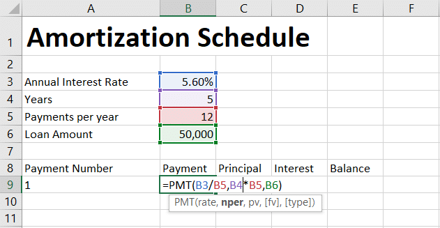
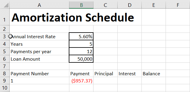
Since this is a payment, Excel automatically will return the result with a negative value of -$957.37.
Step 2: Calculate Principle
Syntax:
=ppmt(rate,per,nper,pv,[fv],[type])We now need to calculate the monthly principle portion of the payment. This is done by using the PPMT Function.
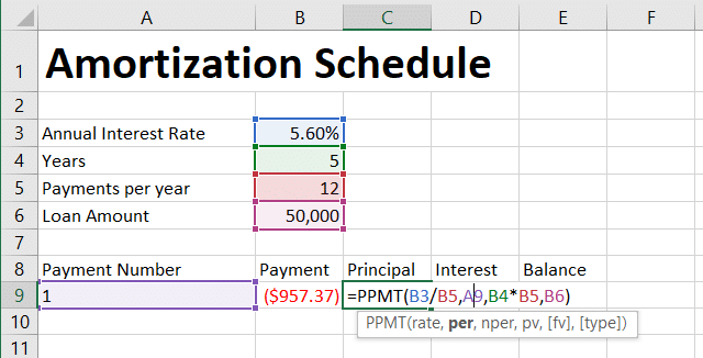
=ppmt(Annual Interest Rate/Payments Per Year,Payment Number,Years of Loan*Payments Per Year,Loan Amount)

=PPMT(B3/B5,A9,B4*B5,B6)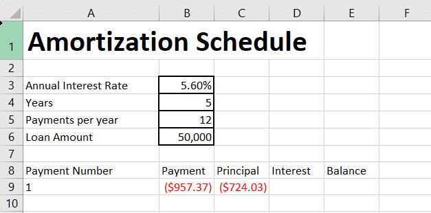
We receive a result of -$724.03 for the first payment.
Step 3: Calculate Interest
Syntax:
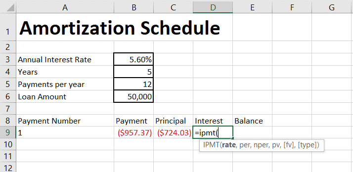
=IPMT(rate,per,nper,pv,[fv],[type])To calculate the interest, we need to use the IPMT Function.
=IPMT(Annual Interest Rate/Payments per year,Payment Number,Years of Loan*Payments Per Year,Loan Amount)

=IPMT(B3/B5,A9,B4*B5,B6)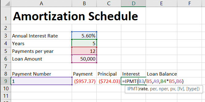
We get a result of -$233.33.
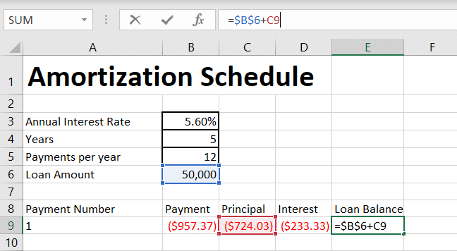
Step 4: Loan Balance for Amortization Schedule
We want to lock the cells with absolute referencing using F4.
We then want to determine the Loan Balance by taking $B$6+C9. Note that we are only locking $B$6.
Let’s finalize the amortization schedule. The following quick video show you how to use the Fill Handle to auto calculate the loan balance.